#import the module we need
from scipy.optimize import curve_fit
import numpy as np
import matplotlib.pyplot as plt
#input data
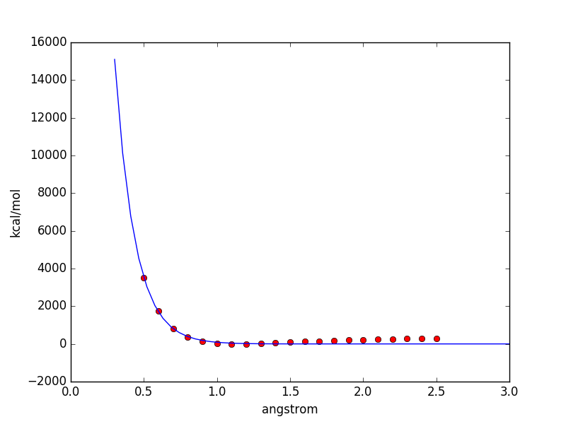
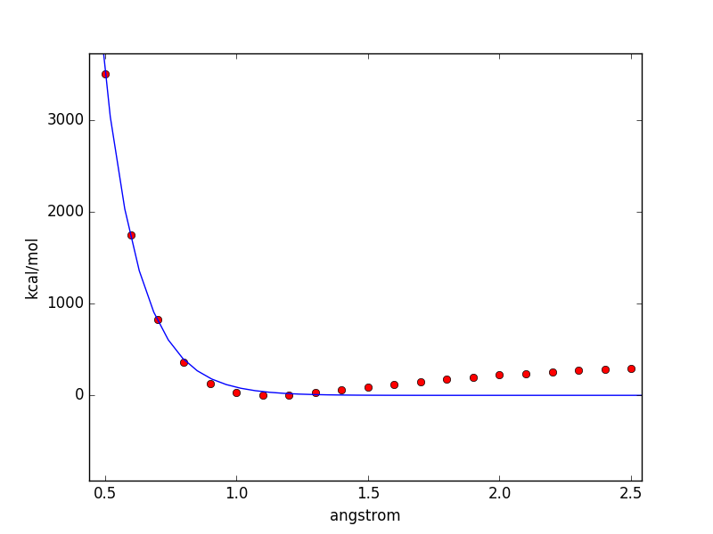
xdata=np.array([0.5,0.6, 0.7, 0.8, 0.9, 1.0 ,1.1 ,1.2 ,1.3 ,1.4 ,1.5 ,1.6 ,1.7 ,1.8 ,1.9 ,2.0 ,2.1 ,2.2 ,2.3 ,2.4 ,2.5])
ydata=[3507.22,1754.07,830.946,359.041,129.637,30.2853,0,5.40111,28.0713,57.9023,89.5626,120.368,149.144,175.434,199.172,220.438,239.392,256.226,271.12,284.256,295.789]
#set the real-line range
t=np.linspace(0.3,3)
def morse(x, D, a, Re, v):
return (D * (np.exp(-2*a*(x-Re))-2*np.exp(-a*(x-Re))) + v)
#using Scipy module
#Parameter
#popt is optimal values for the parameters so that the sum of the squared error of f(xdata, *popt) - ydata is minimized
#pconv is the estimated covariance of popt. the diagonals provide the variance of the parameter estimate.
#p0 means Initial guess for the parameters. If none, then the initial values will all be 1.
#maxfev is the maximum iteration number
tstart = [60, 1, 3, 0]
popt, pcov = curve_fit(morse, xdata, ydata, p0 = tstart, maxfev=5000)
print popt #see the parameter of Morse_Potential
yfit = morse(t,popt[0], popt[1], popt[2], popt[3]) #generating the fitting y value
plt.plot(xdata, ydata,"ro") #plot the original data using 'ro' type
plt.plot(t, yfit) #plot the fitting result
plt.xlabel('angstrom')
plt.ylabel('kcal/mol')
plt.show()